Getting Started with `pyGAM`¶

Introduction¶

Generalized Additive Models (GAMs) are smooth semi-parametric models of the form:

\[g(\mathbb{E}[y|X]) = \beta_0 + f_1(X_1) + f_2(X_2) + \ldots + f_p(X_p)\]

where X.T = [X_1, X_2, ..., X_p] are independent variables, y is the dependent variable, and g() is the link function that relates our predictor variables to the expected value of the dependent variable.

The feature functions f_i() are built using penalized B splines, which allow us to automatically model non-linear relationships without having to manually try out many different transformations on each variable.

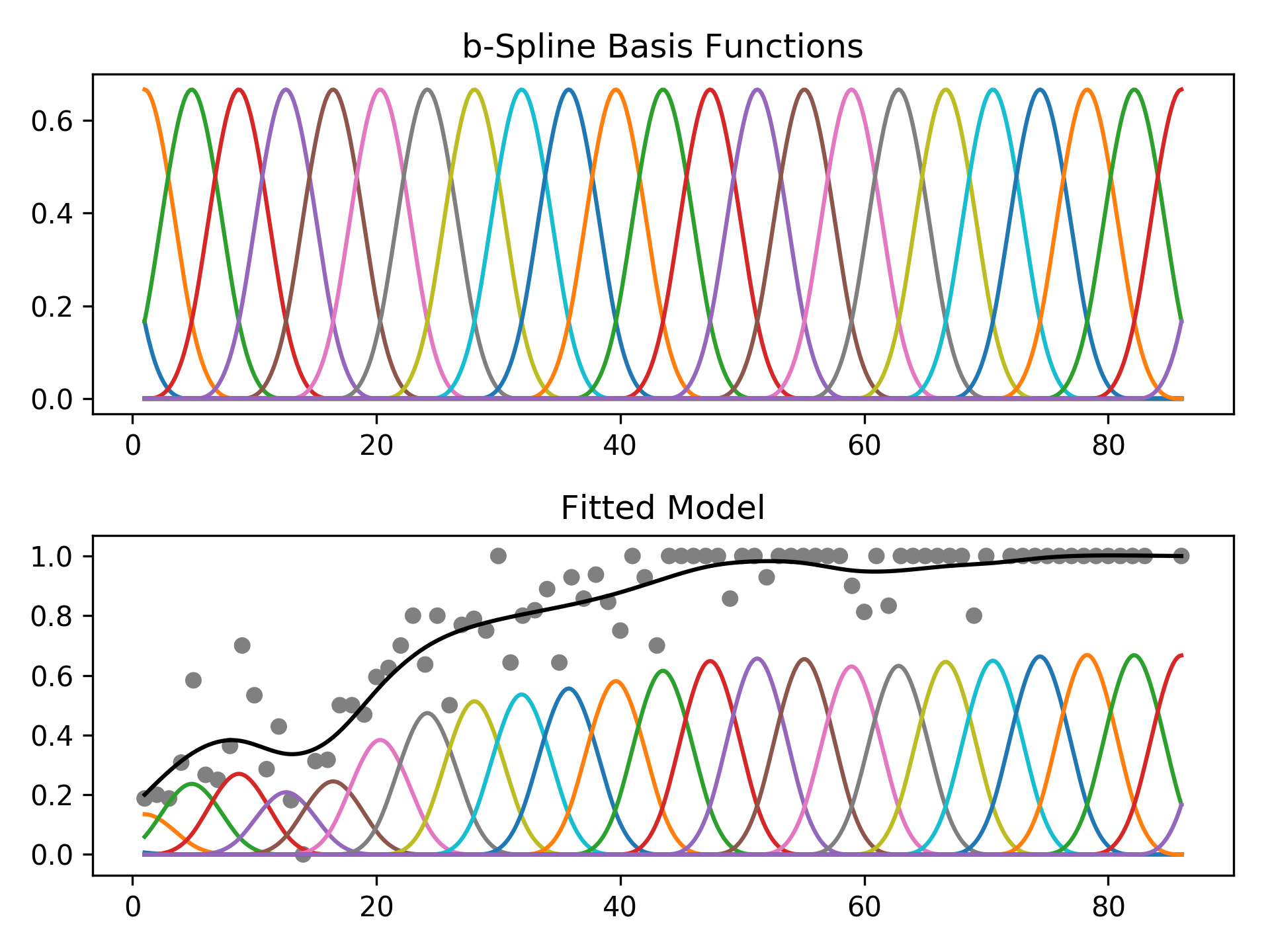
Basis splines

GAMs extend generalized linear models by allowing non-linear functions of features while maintaining additivity. Since the model is additive, it is easy to examine the effect of each X_i on Y individually while holding all other predictors constant.

The result is a very flexible model, where it is easy to incorporate prior knowledge and control overfitting.

Regression¶

For regression problems, we can use a linear GAM which models:

\[\mathbb{E}[y|X]=\beta_0+f_1(X_1)+f_2(X_2)+\dots+f_p(X_p)\]

In [1]:

import matplotlib.pyplot as plt

In [2]:

plt.ion()
plt.rcParams['figure.figsize'] = (12, 8)

In [3]:

from pygam import LinearGAM
from pygam.datasets import wage

X, y = wage(return_X_y=True)

gam = LinearGAM(n_splines=10).gridsearch(X, y)
XX = gam.generate_X_grid()

fig, axs = plt.subplots(1, 3)
titles = ['year', 'age', 'education']

for i, ax in enumerate(axs):
    pdep, confi = gam.partial_dependence(XX, feature=i, width=.95)

    ax.plot(XX[:, i], pdep)
    ax.plot(XX[:, i], *confi, c='r', ls='--')
    ax.set_title(titles[i])

100% (11 of 11) |########################| Elapsed Time: 0:00:01 Time:  0:00:01

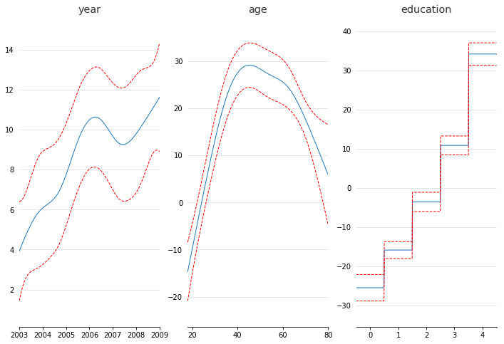
../_images/notebooks_getting_started_4_1.png

Even though we allowed n_splines=10 per numerical feature, our smoothing penalty reduces us to just 14 effective degrees of freedom:

In [4]:

gam.summary()

LinearGAM
=============================================== ==========================================================
Distribution:                        NormalDist Effective DoF:                                      13.532
Link Function:                     IdentityLink Log Likelihood:                                -24119.2327
Number of Samples:                         3000 AIC:                                            48267.5293
                                                AICc:                                           48267.6805
                                                GCV:                                             1247.0706
                                                Scale:                                           1236.9495
                                                Pseudo R-Squared:                                   0.2926
==========================================================================================================
Feature Function   Data Type      Num Splines   Spline Order  Linear Fit  Lambda     P > x      Sig. Code
================== ============== ============= ============= =========== ========== ========== ==========
feature 1          numerical      10            3             False       15.8489    8.23e-03   **
feature 2          numerical      10            3             False       15.8489    1.11e-16   ***
feature 3          categorical    5             0             False       15.8489    1.11e-16   ***
intercept                                                                            1.11e-16   ***
==========================================================================================================
Significance codes:  0 '***' 0.001 '**' 0.01 '*' 0.05 '.' 0.1 ' ' 1

WARNING: Fitting splines and a linear function to a feature introduces a model identifiability problem
         which can cause p-values to appear significant when they are not.

WARNING: p-values calculated in this manner behave correctly for un-penalized models or models with
         known smoothing parameters, but when smoothing parameters have been estimated, the p-values
         are typically lower than they should be, meaning that the tests reject the null too readily.

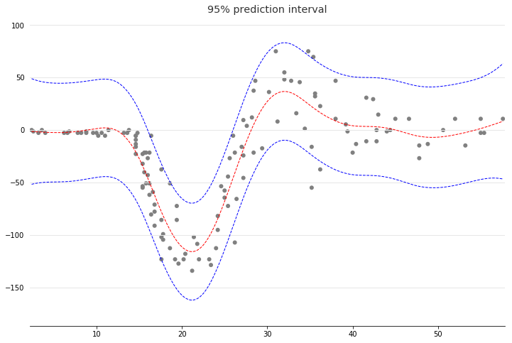
With LinearGAMs, we can also check the prediction intervals:

In [5]:

from pygam.datasets import mcycle

X, y = mcycle(return_X_y=True)

gam = LinearGAM().gridsearch(X, y)
XX = gam.generate_X_grid()

plt.plot(XX, gam.predict(XX), 'r--')
plt.plot(XX, gam.prediction_intervals(XX, width=.95), color='b', ls='--')

plt.scatter(X, y, facecolor='gray', edgecolors='none')
plt.title('95% prediction interval')

100% (11 of 11) |########################| Elapsed Time: 0:00:00 Time:  0:00:00

Out[5]:

Text(0.5,1,'95% prediction interval')

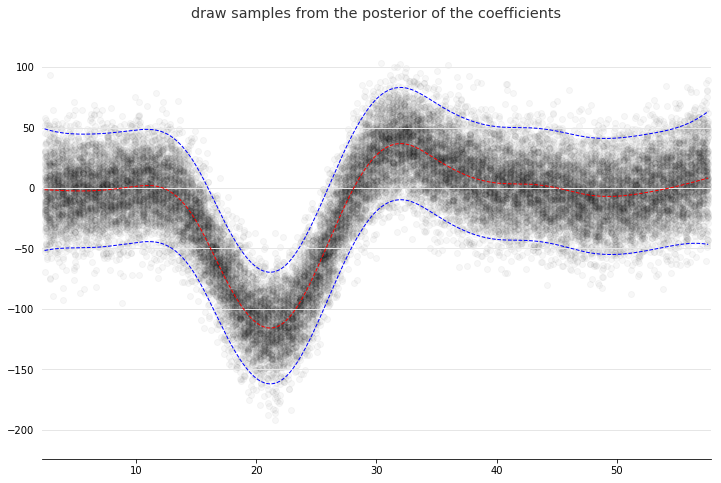
../_images/notebooks_getting_started_8_2.png

And simulate from the posterior:

In [6]:

# continuing last example with the mcycle dataset
for response in gam.sample(X, y, quantity='y', n_draws=50, sample_at_X=XX):
    plt.scatter(XX, response, alpha=.03, color='k')
plt.plot(XX, gam.predict(XX), 'r--')
plt.plot(XX, gam.prediction_intervals(XX, width=.95), color='b', ls='--')
plt.title('draw samples from the posterior of the coefficients')

Out[6]:

Text(0.5,1,'draw samples from the posterior of the coefficients')

../_images/notebooks_getting_started_10_1.png

Classification¶

For binary classification problems, we can use a logistic GAM which models:

\[log\left(\frac{P(y=1|X)}{P(y=0|X)}\right)=\beta_0+f_1(X_1)+f_2(X_2)+\dots+f_p(X_p)\]

In [7]:

from pygam import LogisticGAM
from pygam.datasets import default

X, y = default(return_X_y=True)

gam = LogisticGAM().gridsearch(X, y)
XX = gam.generate_X_grid()

fig, axs = plt.subplots(1, 3)
titles = ['student', 'balance', 'income']

for i, ax in enumerate(axs):
    pdep, confi = gam.partial_dependence(XX, feature=i, width=.95)

    ax.plot(XX[:, i], pdep)
    ax.plot(XX[:, i], confi[0], c='r', ls='--')
    ax.set_title(titles[i])

100% (11 of 11) |########################| Elapsed Time: 0:00:07 Time:  0:00:07

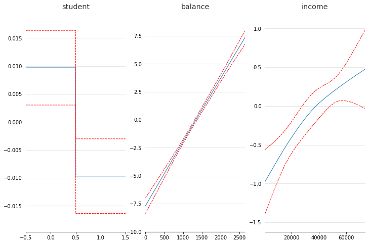
../_images/notebooks_getting_started_12_1.png

We can then check the accuracy:

In [8]:

gam.accuracy(X, y)

Out[8]:

0.9739

Since the scale of the Binomial distribution is known, our gridsearch minimizes the Un-Biased Risk Estimator (UBRE) objective:

In [9]:

gam.summary()

LogisticGAM
=============================================== ==========================================================
Distribution:                      BinomialDist Effective DoF:                                      4.3643
Link Function:                        LogitLink Log Likelihood:                                  -788.7121
Number of Samples:                        10000 AIC:                                             1586.1527
                                                AICc:                                            1586.1595
                                                UBRE:                                                2.159
                                                Scale:                                                 1.0
                                                Pseudo R-Squared:                                   0.4599
==========================================================================================================
Feature Function   Data Type      Num Splines   Spline Order  Linear Fit  Lambda     P > x      Sig. Code
================== ============== ============= ============= =========== ========== ========== ==========
feature 1          categorical    2             0             False       1000.0     4.41e-03   **
feature 2          numerical      25            3             False       1000.0     0.00e+00   ***
feature 3          numerical      25            3             False       1000.0     2.35e-02   *
intercept                                                                            0.00e+00   ***
==========================================================================================================
Significance codes:  0 '***' 0.001 '**' 0.01 '*' 0.05 '.' 0.1 ' ' 1

WARNING: Fitting splines and a linear function to a feature introduces a model identifiability problem
         which can cause p-values to appear significant when they are not.

WARNING: p-values calculated in this manner behave correctly for un-penalized models or models with
         known smoothing parameters, but when smoothing parameters have been estimated, the p-values
         are typically lower than they should be, meaning that the tests reject the null too readily.

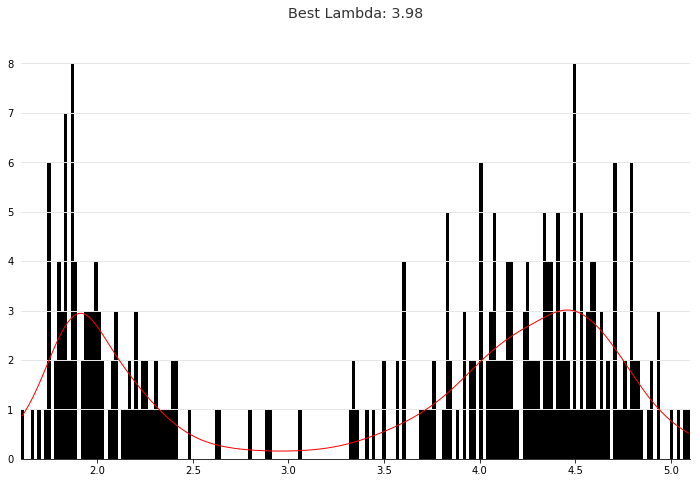
Poisson and Histogram Smoothing¶

We can intuitively perform histogram smoothing by modeling the counts in each bin as being distributed Poisson via PoissonGAM.

In [10]:

from pygam import PoissonGAM
from pygam.datasets import faithful

X, y = faithful(return_X_y=True)

gam = PoissonGAM().gridsearch(X, y)

plt.hist(faithful(return_X_y=False)['eruptions'], bins=200, color='k');
plt.plot(X, gam.predict(X), color='r')
plt.title('Best Lambda: {0:.2f}'.format(gam.lam))

100% (11 of 11) |########################| Elapsed Time: 0:00:00 Time:  0:00:00

Out[10]:

Text(0.5,1,'Best Lambda: 3.98')

../_images/notebooks_getting_started_18_2.png

Custom Models¶

It’s also easy to build custom models, by using the base GAM class and specifying the distribution and the link function.`

In [11]:

from pygam import GAM
from pygam.datasets import trees

X, y = trees(return_X_y=True)

gam = GAM(distribution='gamma', link='log', n_splines=4)
gam.gridsearch(X, y)

plt.scatter(y, gam.predict(X))
plt.xlabel('true volume')
plt.ylabel('predicted volume')

100% (11 of 11) |########################| Elapsed Time: 0:00:00 Time:  0:00:00

Out[11]:

Text(0,0.5,'predicted volume')

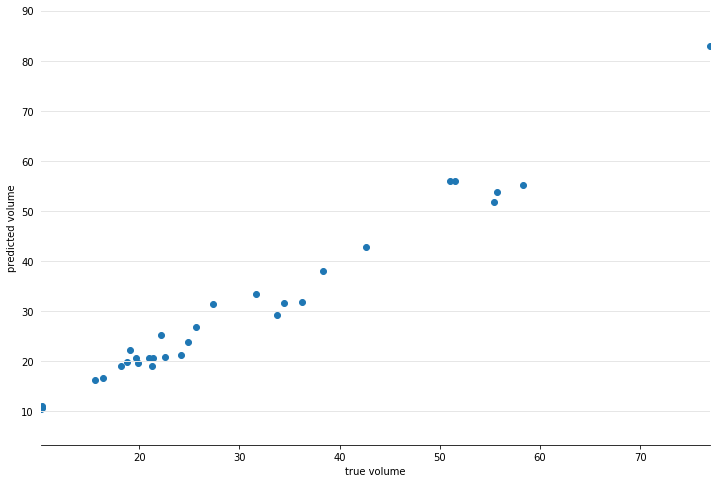
../_images/notebooks_getting_started_20_2.png

We can check the quality of the fit by looking at the Pseudo R-Squared:

In [12]:

gam.summary()

GAM
=============================================== ==========================================================
Distribution:                         GammaDist Effective DoF:                                      4.1544
Link Function:                          LogLink Log Likelihood:                                   -66.9372
Number of Samples:                           31 AIC:                                              144.1832
                                                AICc:                                             146.7368
                                                GCV:                                                0.0095
                                                Scale:                                              0.0073
                                                Pseudo R-Squared:                                   0.9767
==========================================================================================================
Feature Function   Data Type      Num Splines   Spline Order  Linear Fit  Lambda     P > x      Sig. Code
================== ============== ============= ============= =========== ========== ========== ==========
feature 1          numerical      4             3             False       0.0158     1.11e-16   ***
feature 2          numerical      4             3             False       0.0158     8.28e-05   ***
intercept                                                                            1.11e-16   ***
==========================================================================================================
Significance codes:  0 '***' 0.001 '**' 0.01 '*' 0.05 '.' 0.1 ' ' 1

WARNING: Fitting splines and a linear function to a feature introduces a model identifiability problem
         which can cause p-values to appear significant when they are not.

WARNING: p-values calculated in this manner behave correctly for un-penalized models or models with
         known smoothing parameters, but when smoothing parameters have been estimated, the p-values
         are typically lower than they should be, meaning that the tests reject the null too readily.

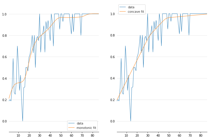
Penalties / Constraints¶

With GAMs we can encode prior knowledge and control overfitting by using penalties and constraints.

Available penalties - second derivative smoothing (default on numerical features) - L2 smoothing (default on categorical features)

Availabe constraints - monotonic increasing/decreasing smoothing - convex/concave smoothing - periodic smoothing [soon…]

We can inject our intuition into our model by using monotonic and concave constraints:

In [13]:

from pygam import LinearGAM
from pygam.datasets import hepatitis

X, y = hepatitis(return_X_y=True)

gam1 = LinearGAM(constraints='monotonic_inc').fit(X, y)
gam2 = LinearGAM(constraints='concave').fit(X, y)

fig, ax = plt.subplots(1, 2)
ax[0].plot(X, y, label='data')
ax[0].plot(X, gam1.predict(X), label='monotonic fit')
ax[0].legend()

ax[1].plot(X, y, label='data')
ax[1].plot(X, gam2.predict(X), label='concave fit')
ax[1].legend()

Out[13]:

<matplotlib.legend.Legend at 0xd9c8550>

../_images/notebooks_getting_started_24_1.png

API¶

pyGAM is intuitive, modular, and adheres to a familiar API:

In [14]:

from pygam import LogisticGAM
from pygam.datasets import toy_classification

X, y = toy_classification(return_X_y=True, n=5000)

gam = LogisticGAM()
gam.fit(X, y)

Out[14]:

LogisticGAM(callbacks=[Deviance(), Diffs(), Accuracy()],
   constraints=None, dtype='auto', fit_intercept=True,
   fit_linear=False, fit_splines=True, lam=0.6, max_iter=100,
   n_splines=25, penalties='auto', spline_order=3, tol=0.0001,
   verbose=False)

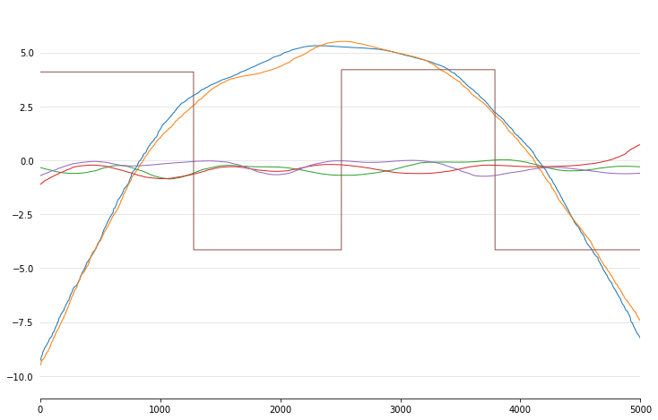
Since GAMs are additive, it is also super easy to visualize each individual feature function, f_i(X_i). These feature functions describe the effect of each X_i on y individually while marginalizing out all other predictors:

In [15]:

import numpy as np

pdeps = gam.partial_dependence(np.sort(X, axis=0))
_ = plt.plot(pdeps)

../_images/notebooks_getting_started_28_0.png

Current Features¶

Models¶

pyGAM comes with many models out-of-the-box:

GAM (base class for constructing custom models)
LinearGAM
LogisticGAM
GammaGAM
PoissonGAM
InvGaussGAM

You can mix and match distributions with link functions to create custom models!

In [16]:

GAM(distribution='gamma', link='inverse')

Out[16]:

GAM(callbacks=['deviance', 'diffs'], constraints=None,
   distribution='gamma', dtype='auto', fit_intercept=True,
   fit_linear=False, fit_splines=True, lam=0.6, link='inverse',
   max_iter=100, n_splines=25, penalties='auto', spline_order=3,
   tol=0.0001, verbose=False)

Distributions¶

Normal
Binomial
Gamma
Poisson
Inverse Gaussian

Link Functions¶

Link functions take the distribution mean to the linear prediction. These are the canonical link functions for the above distributions:

Identity
Logit
Inverse
Log
Inverse-squared

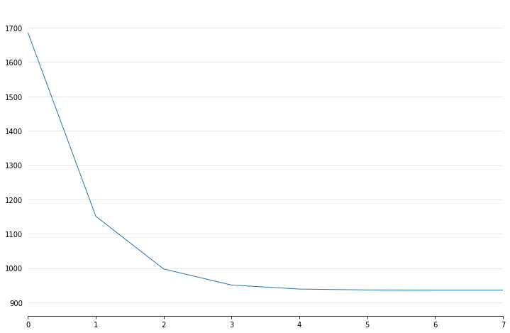
Callbacks¶

Callbacks are performed during each optimization iteration. It’s also easy to write your own.

deviance - model deviance
diffs - differences of coefficient norm
accuracy - model accuracy for LogisticGAM
coef - coefficient logging

You can check a callback by inspecting:

In [17]:

_ = plt.plot(gam.logs_['deviance'])

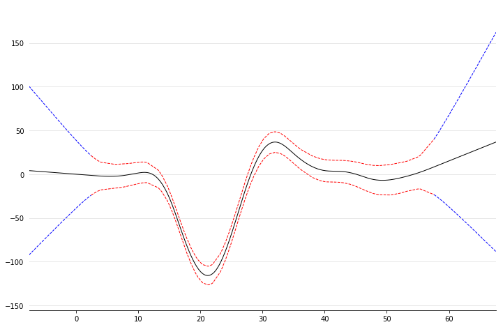
../_images/notebooks_getting_started_32_0.png

Linear Extrapolation¶

In [18]:

X, y = mcycle()

gam = LinearGAM()
gam.gridsearch(X, y)

XX = gam.generate_X_grid()

m = X.min()
M = X.max()
XX = np.linspace(m - 10, M + 10, 500)
Xl = np.linspace(m - 10, m, 50)
Xr = np.linspace(M, M + 10, 50)

plt.figure()

plt.plot(XX, gam.predict(XX), 'k')
plt.plot(Xl, gam.confidence_intervals(Xl), color='b', ls='--')
plt.plot(Xr, gam.confidence_intervals(Xr), color='b', ls='--')
_ = plt.plot(X, gam.confidence_intervals(X), color='r', ls='--')

100% (11 of 11) |########################| Elapsed Time: 0:00:00 Time:  0:00:00

../_images/notebooks_getting_started_34_1.png

Citing pyGAM¶

Please consider citing pyGAM if it has helped you in your research or work:

Daniel Servén, & Charlie Brummitt. (2018, March 27). pyGAM: Generalized Additive Models in Python. Zenodo. DOI: 10.5281/zenodo.1208723

BibTex:

@misc{daniel\_serven\_2018_1208723,
  author       = {Daniel Servén and
                  Charlie Brummitt},
  title        = {pyGAM: Generalized Additive Models in Python},
  month        = mar,
  year         = 2018,
  doi          = {10.5281/zenodo.1208723},
  url          = {https://doi.org/10.5281/zenodo.1208723}
}

References¶

Simon N. Wood, 2006

Generalized Additive Models: an introduction with R
Hastie, Tibshirani, Friedman

The Elements of Statistical Learning

http://statweb.stanford.edu/~tibs/ElemStatLearn/printings/ESLII_print10.pdf
James, Witten, Hastie and Tibshirani

An Introduction to Statistical Learning

http://www-bcf.usc.edu/~gareth/ISL/ISLR%20Sixth%20Printing.pdf
Paul Eilers & Brian Marx, 1996 Flexible Smoothing with B-splines and Penalties http://www.stat.washington.edu/courses/stat527/s13/readings/EilersMarx_StatSci_1996.pdf
Kim Larsen, 2015

GAM: The Predictive Modeling Silver Bullet

http://multithreaded.stitchfix.com/assets/files/gam.pdf
Deva Ramanan, 2008

UCI Machine Learning: Notes on IRLS

http://www.ics.uci.edu/~dramanan/teaching/ics273a_winter08/homework/irls_notes.pdf
Paul Eilers & Brian Marx, 2015

International Biometric Society: A Crash Course on P-splines

http://www.ibschannel2015.nl/project/userfiles/Crash_course_handout.pdf
Keiding, Niels, 1991

Age-specific incidence and prevalence: a statistical perspective

Getting Started with pyGAM¶